DeepSeek V4.1 CED and CSA2 Architecture Notes

TL;DR

• DeepSeek V4.1-Flash is still an autoregressive causal language model, but its 40 Transformer blocks are split into a 20-layer causal encoder and a 20-layer decoder.
• The causal encoder processes the full prompt and produces H20, a sequence of per-position hidden states. H20 is not one pooled vector and is not the twentieth token.
• Decoder global KV is projected from H20. In the released CSA2 schedule, decoder layer 20 owns the shared global KV, while later decoder layers reuse it.
• Every decoder layer still computes its own query, attention output, and layer-local sliding-window KV. Sharing global KV does not mean copying an earlier layer's attention output.
• CED primarily improves inference prefill. CSA2 improves both training and inference, but its largest deployment benefit is reducing KV-cache capacity, indexing work, memory traffic, and persistent cache storage.
• Unlike DeepSeek V4, which alternates CSA and HCA, DeepSeek V4.1-Flash uses pure CSA2 for its global attention path.

1. From DSA to CSA2

The three mechanisms are best understood as successive reductions along the sequence and layer dimensions.

Mechanism	Candidate representation	Sparse selection	Cross-layer reuse	Main purpose
DSA	One original KV entry per token	Select top-k original token entries	No	Reduce core-attention work
CSA	Learned compressed KV entries	Select top-k compressed entries	No	Reduce core-attention work, indexer work, and KV size
CSA2	Simplified compressed KV entries	Select or reuse top-k compressed entries	Main KV, indexer K, and top-k indices	Reduce work and cache duplication across both sequence and layer dimensions

For a sequence of length N and compression ratio m, DSA indexes roughly N token entries, while CSA and CSA2 index roughly N / m compressed entries. CSA can therefore be summarized as "compress, then apply sparse attention." CSA2 adds layer-dimension sharing on top of that design.

2. CED versus a traditional decoder-only stack

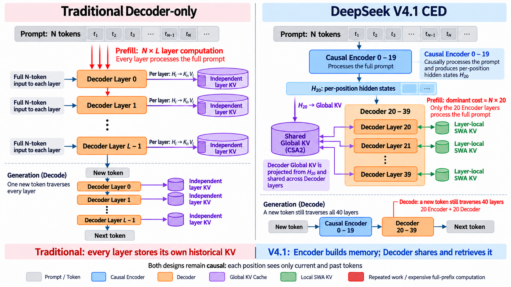
A conventional decoder-only model uses a homogeneous stack. During prefill, every prompt position traverses every layer, and every layer derives its own KV history from its own hidden states.

DeepSeek V4.1-Flash instead divides the backbone into:

Layer range, zero-based	Role	Full-prompt responsibility
0-19	Causal encoder	Processes the full prompt and produces H20
20-39	Decoder	Retrieves global memory derived from H20 and maintains layer-local SWA state

Both halves remain causal. This is not a BERT-style bidirectional encoder and not a traditional T5-style encoder-decoder system. At position t, the encoder representation can depend only on positions up to t.

3. What H20 means

Let H0 be the token embedding sequence. With zero-based block numbering:

block 0:  H0  -> H1
block 1:  H1  -> H2
...
block 19: H19 -> H20

For batch size B, sequence length N, and hidden dimension d, the boundary state is a sequence tensor:

\[ H_{20} \in \mathbb{R}^{B \times N \times d}. \]

Each row H20[t] is the causal representation of the prefix ending at position t. The model preserves one representation per sequence position rather than pooling the prompt into one vector.

The decoder global memory is derived from this boundary state:

\[ C^{\mathrm{global}} = f_{\mathrm{KV}}(H_{20}). \]

The exact path also includes CSA2 compression when the configured ratio is greater than one, quantization, and indexer-K projection.

4. Does the decoder have its own KV?

The answer depends on which KV path is meant.

Quantity	Source	Shared across decoder layers?
Main query	Current decoder layer hidden state	No
Long-range global KV	Projected from H20; owned by the decoder Full layer	Yes
Indexer K	Projected from the shared main KV	Yes
Top-k indices	Produced by Full/Reindex or reused by Reuse	Shared within each index group
Local SWA KV	Current decoder layer hidden state	No

Conceptually, decoder layer l performs:

\[ Q_l = f^Q_l(H_l), \]

followed by attention over both selected global entries and the layer's own local sliding-window state:

\[ O_l = \mathrm{Attention} \left( Q_l, \left[ C^{\mathrm{global}}_{\mathrm{selected}}; C^{\mathrm{SWA}}_l \right] \right). \]

The decoder therefore does not keep one independent long-range global KV cache per layer, but it does keep independent layer-local SWA KV. Every layer also produces a new query and a new attention output. A decoder query attends to KV projected from H20, not directly to the raw H20 tensor.

5. The three CSA2 modes

All three modes compute a layer-specific main query, layer-local SWA KV, sparse attention, and output projection. They differ only in how they obtain global KV, indexer state, and sparse positions.

Mode	Main KV and indexer K	Top-k selection	Work saved
Full	Generated by the current layer	Fresh indexer evaluation	None; this is the owner/source layer
Reindex	Reused from the latest Full layer	Fresh selection using this layer's indexer Q	Avoids a new global KV cache while allowing retrieval to change with depth
Reuse	Reused from the latest Full layer	Reuses the latest compatible Full/Reindex selection	Avoids both KV generation and indexer evaluation

Reuse does not skip attention. It reuses the memory and selected positions, but the current layer still assigns its own attention weights and produces its own output.

6. Released V4.1-Flash layer schedule

The released configuration statically assigns the modes as follows:

Layers	Section	Compression ratio	Mode pattern
0-1	Encoder	None	SWA only
2-7	Encoder	2	Full + 5 Reuse
8-13	Encoder	2	Full + 5 Reuse
14-19	Encoder	2	Full + 5 Reuse
20-23	Decoder	1	Full + 3 Reuse
24-27	Decoder	1	Reindex + 3 Reuse
28-31	Decoder	1	Reindex + 3 Reuse
32-35	Decoder	1	Reindex + 3 Reuse
36-39	Decoder	1	Reindex + 3 Reuse

The four global-KV owners are layers 2, 8, 14, and 20. The index-source layers are 2, 8, 14, 20, 24, 28, 32, and 36. This yields:

• 2 SWA-only layers;
• 4 Full layers;
• 4 Reindex layers; and
• 30 Reuse layers.

The encoder compresses pairs of positions into global entries. The decoder uses compression ratio one: it does not merge adjacent positions, but it still benefits from sparse selection, cross-layer KV sharing, index reuse, and FP4 global-KV storage.

7. Hierarchical indexing in the decoder

Decoder layer 20 is the only decoder Full layer. It scans the full causally visible global history, chooses its final top-512 entries, and also builds a larger candidate pool for later Reindex layers.

The released settings use 2,048 selected blocks with eight positions per block, producing at most 16,384 candidate positions. Layers 24, 28, 32, and 36 select their own top-512 entries from this bounded pool rather than rescanning the entire context. The three Reuse layers after each index-producing layer reuse that layer's top-512 selection.

The first decoder indexer still scales with context length. The deeper Reindex layers have a bounded search domain once the candidate-pool size is fixed.

8. Training versus inference benefits

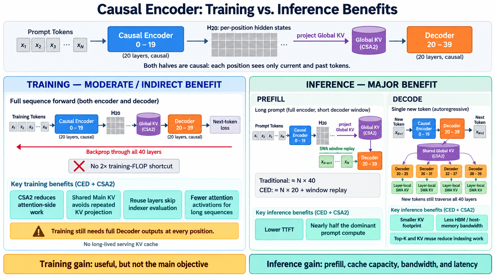
Training

Standard next-token training needs a final decoder output at every sequence position, followed by backward propagation through the complete network. CED therefore does not provide the same near-2x shortcut that it provides for inference prefill.

Training can still benefit from CSA2 because:

• compressed and sparse attention reduces attention-side work on long sequences;
• shared main KV avoids repeated KV projections;
• Reuse layers avoid new indexer evaluations; and
• fewer attention-side intermediates may need to be retained or recomputed.

These gains are not free. In pipeline-parallel training, source and consumer layers can reside on different stages, so DeepSeek uses shadow indexers, cross-stage payloads, gradient synchronization, and microbatch-level shared state management.

Training activations should also not be confused with a serving KV cache. Training tensors generally live for a forward/backward step, whereas an inference KV cache persists across autoregressive generation steps and may be stored in HBM, host memory, or SSD for prefix reuse.

Inference prefill

For a long prompt, a traditional 40-layer decoder-only model performs roughly N x 40 layer-token work. CED lets the full prompt primarily traverse the 20-layer causal encoder. Decoder global KV is projected from H20, while the decoder SWA path replays only a bounded recent window.

The dominant long-prompt work is therefore approximately:

\[ N \times 20 + n_{\mathrm{win}} \times 20, \]

which approaches N x 20 when the prompt is much longer than the local window. This is primarily a time-to-first-token and prompt-processing optimization.

Autoregressive decode

Each newly generated token still traverses all 40 backbone layers. CED does not turn decode into a 20-layer path. The deployment benefits instead come from:

• shared global KV rather than one independent long-range cache per decoder layer;
• FP4 global-KV storage;
• top-k sparse reads;
• bounded candidate searches for deeper Reindex layers;
• index reuse in Reuse layers; and
• small layer-local SWA caches.

DeepSeek reports a global KV footprint of 890 bytes per token, about one quarter of DeepSeek V4-Flash at the same sequence length. SWA Bounded Replay further reduces persistent cache storage to roughly one eighth of V4-Flash by avoiding the need to persist the full layer-wise SWA state.

9. Practical mental model

A useful summary is:

causal encoder = build a reusable per-position memory representation
decoder       = query that global memory and maintain local layer state
CSA2          = compress, sparsify, and share the global memory across layers

Or, in terms of what each mechanism primarily saves:

CED           -> long-prompt prefill compute
CSA2          -> attention work, indexer work, and cross-layer KV duplication
FP4 global KV -> cache capacity and memory bandwidth
bounded replay-> persistent SWA-cache storage

References

• DeepSeek-V4.1-Flash: Pushing the Limits of KV Cache Compression
• DeepSeek-V4.1-Flash model and inference configuration
• DeepSeek-V4: Towards Highly Efficient Million-Token Context Intelligence
• DeepSeek-V3.2: Pushing the Frontier of Open Large Language Models